Tag Archives: PCGuide

Hard Disk Operational Overview

As an illustration, I’ll describe here in words how the various components in the disk interoperate when they receive a request for data. Hopefully this will provide some context for the descriptions of the components that follow in later sections.

A hard disk uses round, flat disks called platters, coated on both sides with a special media material designed to store information in the form of magnetic patterns. The platters are mounted by cutting a hole in the center and stacking them onto a spindle. The platters rotate at high speed, driven by a special spindle motor connected to the spindle. Special electromagnetic read/write devices called heads are mounted onto sliders and used to either record information onto the disk or read information from it. The sliders are mounted onto arms, all of which are mechanically connected into a single assembly and positioned over the surface of the disk by a device called an actuator. A logic board controls the activity of the other components and communicates with the rest of the PC.

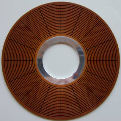
Each surface of each platter on the disk can hold tens of billions of individual bits of data. These are organized into larger “chunks” for convenience, and to allow for easier and faster access to information. Each platter has two heads, one on the top of the platter and one on the bottom, so a hard disk with three platters (normally) has six surfaces and six total heads. Each platter has its information recorded in concentric circles called tracks. Each track is further broken down into smaller pieces called sectors, each of which holds 512 bytes of information.

The entire hard disk must be manufactured to a high degree of precision due to the extreme miniaturization of the components, and the importance of the hard disk’s role in the PC. The main part of the disk is isolated from outside air to ensure that no contaminants get onto the platters, which could cause damage to the read/write heads.

Exploded view of a hard drive
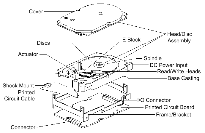
Exploded line drawing of a modern hard disk, showing the major components.
Though the specifics vary greatly between different designs, the basic
components you see above are typical of almost all PC hard disks.
Original image © Seagate Technology Image used with permission.

Here’s an example case showing in brief what happens in the disk each time a piece of information needs to be read from it. This is a highly simplified example because it ignores factors such as disk caching, error correction, and many of the other special techniques that systems use today to increase performance and reliability. For example, sectors are not read individually on most PCs; they are grouped together into continuous chunks called clusters. A typical job, such as loading a file into a spreadsheet program, can involve thousands or even millions of individual disk accesses, and loading a 20 MB file 512 bytes at a time would be rather inefficient:

  1. The first step in accessing the disk is to figure out where on the disk to look for the needed information. Between them, the application, operating system, system BIOS and possibly any special driver software for the disk, do the job of determining what part of the disk to read.
  2. The location on the disk undergoes one or more translation steps until a final request can be made to the drive with an address expressed in terms of its geometry. The geometry of the drive is normally expressed in terms of the cylinder, head and sector that the system wants the drive to read. (A cylinder is equivalent to a track for addressing purposes). A request is sent to the drive over the disk drive interface giving it this address and asking for the sector to be read.
  3. The hard disk’s control program first checks to see if the information requested is already in the hard disk’s own internal buffer (or cache). It if is then the controller supplies the information immediately, without needing to look on the surface of the disk itself.
  4. In most cases the disk drive is already spinning. If it isn’t (because power management has instructed the disk to “spin down” to save energy) then the drive’s controller board will activate the spindle motor to “spin up” the drive to operating speed.
  5. The controller board interprets the address it received for the read, and performs any necessary additional translation steps that take into account the particular characteristics of the drive. The hard disk’s logic program then looks at the final number of the cylinder requested. The cylinder number tells the disk which track to look at on the surface of the disk. The board instructs the actuator to move the read/write heads to the appropriate track.
  6. When the heads are in the correct position, the controller activates the head specified in the correct read location. The head begins reading the track looking for the sector that was asked for. It waits for the disk to rotate the correct sector number under itself, and then reads the contents of the sector.
  7. The controller board coordinates the flow of information from the hard disk into a temporary storage area (buffer). It then sends the information over the hard disk interface, usually to the system memory, satisfying the system’s request for data.

The PC Guide
Site Version: 2.2.0 – Version Date: April 17, 2001
© Copyright 1997-2004 Charles M. Kozierok. All Rights Reserved.

This is an archive of Charles M. Kozierok’s PCGuide (pcguide.com) which disappeared from the internet in 2018. We wanted to preserve Charles M. Kozierok’s knowledge about computers and are permanently hosting a selection of important pages from PCGuide.

Hard Disk Platters and Media

Every hard disk contains one or more flat disks that are used to actually hold the data in the drive. These disks are called platters (sometimes also “disks” or “discs”). They are composed of two main substances: a substrate material that forms the bulk of the platter and gives it structure and rigidity, and a magnetic media coating which actually holds the magnetic impulses that represent the data. Hard disks get their name from the rigidity of the platters used, as compared to floppy disks and other media which use flexible “platters” (actually, they aren’t usually even called platters when the material is flexible.)

The platters are “where the action is”–this is where the data itself is recorded. For this reason the quality of the platters and particularly, their media coating, is critical. The surfaces of each platter are precision machined and treated to remove any imperfections, and the hard disk itself is assembled in a clean room to reduce the chances of any dirt or contamination getting onto the platters.


The PC Guide
Site Version: 2.2.0 – Version Date: April 17, 2001
© Copyright 1997-2004 Charles M. Kozierok. All Rights Reserved.

This is an archive of Charles M. Kozierok’s PCGuide (pcguide.com) which disappeared from the internet in 2018. We wanted to preserve Charles M. Kozierok’s knowledge about computers and are permanently hosting a selection of important pages from PCGuide.

Hard Disk Tracks, Cylinders and Sectors

All information stored on a hard disk is recorded in tracks, which are concentric circles placed on the surface of each platter, much like the annual rings of a tree. The tracks are numbered, starting from zero, starting at the outside of the platter and increasing as you go in. A modern hard disk has tens of thousands of tracks on each platter.

5.25" hard disk platter
A platter from a 5.25″ hard disk, with 20 concentric tracks drawn
over the surface. Each track is divided into 16 imaginary sectors.

Data is accessed by moving the heads from the inner to the outer part of the disk, driven by the head actuator. This organization of data allows for easy access to any part of the disk, which is why disks are called random access storage devices.

Each track can hold many thousands of bytes of data. It would be wasteful to make a track the smallest unit of storage on the disk, since this would mean small files wasted a large amount of space. Therefore, each track is broken into smaller units called sectors. Each sector holds 512 bytes of user data, plus as many as a few dozen additional bytes used for internal drive control and for error detection and correction.


The PC Guide
Site Version: 2.2.0 – Version Date: April 17, 2001
© Copyright 1997-2004 Charles M. Kozierok. All Rights Reserved.

This is an archive of Charles M. Kozierok’s PCGuide (pcguide.com) which disappeared from the internet in 2018. We wanted to preserve Charles M. Kozierok’s knowledge about computers and are permanently hosting a selection of important pages from PCGuide.

Hard Drive Sector Format and Structure

The basic unit of data storage on a hard disk is the sector. The name “sector” comes from the mathematical term, which refers to a “pie-shaped” angular section of a circle, bounded on two sides by radii and the third by the perimeter of the circle. On a hard disk containing concentric circular tracks, that shape would define a sector of each track of the platter surface that it intercepted. This is what is called a sector in the hard disk world: a small segment along the length of a track. At one time, all hard disks had the same number of sectors per track, and in fact, the number of sectors in each track was fairly standard between models. Today’s advances have allowed the number of sectors per track (“SPT”) to vary significantly, as discussed here.

In the PC world, each sector of a hard disk can store 512 bytes of user data. (There are some disks where this number can be modified, but 512 is the standard, and found on virtually all hard drives by default.) Each sector, however, actually holds much more than 512 bytes of information. Additional bytes are needed for control structures and other information necessary to manage the drive, locate data and perform other “support functions”. The exact details of how a sector is structured depends on the drive model and manufacturer. However, the contents of a sector usually include the following general elements:

  • ID Information: Conventionally, space is left in each sector to identify the sector’s number and location. This is used for locating the sector on the disk. Also included in this area is status information about the sector. For example, a bit is commonly used to indicate if the sector has been marked defective and remapped.
  • Synchronization Fields: These are used internally by the drive controller to guide the read process.
  • Data: The actual data in the sector.
  • ECC: Error correcting code used to ensure data integrity.
  • Gaps: One or more “spacers” added as necessary to separate other areas of the sector, or provide time for the controller to process what it has read before reading more bits.

Note: In addition to the sectors, each containing the items above, space on each track is also used for servo information (on embedded servo drives, which is the design used by all modern units).

The amount of space taken up by each sector for overhead items is important, because the more bits used for “management”, the fewer overall that can be used for data. Therefore, hard disk manufacturers strive to reduce the amount of non-user-data information that must be stored on the disk. The term format efficiency refers to the percentage of bits on each disk that are used for data, as opposed to “other things”. The higher the format efficiency of a drive, the better (but don’t expect to find statistics on this for your favorite drive easy to find!)

One of the most important improvements in sector format was IBM’s creation of the No-ID Format in the mid-1990s. The idea behind this innovation is betrayed by the name: the ID fields are removed from the sector format. Instead of labeling each sector within the sector header itself, a format map is stored in memory and referenced when a sector must be located. This map also contains information about what sectors have been marked bad and relocated, where the sectors are relative to the location of servo information, and so on. Not only does this improve format efficiency, allowing up to 10% more data to be stored on the surface of each platter, it also improves performance. Since this critical positioning information is present in high-speed memory, it can be accessed much more quickly. “Detours” in chasing down remapped sectors are also eliminated.


The PC Guide
Site Version: 2.2.0 – Version Date: April 17, 2001
© Copyright 1997-2004 Charles M. Kozierok. All Rights Reserved.

This is an archive of Charles M. Kozierok’s PCGuide (pcguide.com) which disappeared from the internet in 2018. We wanted to preserve Charles M. Kozierok’s knowledge about computers and are permanently hosting a selection of important pages from PCGuide.

Hard Drive Error Correcting Code (ECC)

The basis of all error detection and correction in hard disks is the inclusion of redundant information and special hardware or software to use it. Each sector of data on the hard disk contains 512 bytes, or 4,096 bits, of user data. In addition to these bits, an additional number of bits are added to each sector for the implementation of error correcting code or ECC (sometimes also called error correction code or error correcting circuits). These bits do not contain data; rather, they contain information about the data that can be used to correct any problems encountered trying to access the real data bits.

There are several different types of error correcting codes that have been invented over the years, but the type commonly used on PCs is the Reed-Solomon algorithm, named for researchers Irving Reed and Gustave Solomon, who first discovered the general technique that the algorithm employs. Reed-Solomon codes are widely used for error detection and correction in various computing and communications media, including magnetic storage, optical storage, high-speed modems, and data transmission channels. They have been chosen because they are easier to decode than most other similar codes, can detect (and correct) large numbers of missing bits of data, and require the least number of extra ECC bits for a given number of data bits. Look in the memory section for much more general information on error detection and correction.

When a sector is written to the hard disk, the appropriate ECC codes are generated and stored in the bits reserved for them. When the sector is read back, the user data read, combined with the ECC bits, can tell the controller if any errors occurred during the read. Errors that can be corrected using the redundant information are corrected before passing the data to the rest of the system. The system can also tell when there is too much damage to the data to correct, and will issue an error notification in that event. The sophisticated firmware present in all modern drives uses ECC as part of its overall error management protocols. This is all done “on the fly” with no intervention from the user required, and no slowdown in performance even when errors are encountered and must be corrected.

The capability of a Reed Solomon ECC implementation is based on the number of additional ECC bits it includes. The more bits that are included for a given amount of data, the more errors that can be tolerated. There are multiple trade offs involved in deciding how many bits of ECC information to use. Including more bits per sector of data allows for more robust error detection and correction, but means fewer sectors can be put on each track, since more of the linear distance of the track is used up with non-data bits. On the other hand, if you make the system more capable of detecting and correcting errors, you make it possible to increase areal density or make other performance improvements, which could pay back the “investment” of extra ECC bits, and then some. Another complicating factor is that the more ECC bits included, the more processing power the controller must possess to process the Reed Solomon algorithm. The engineers who design hard disks take these various factors into account in deciding how many ECC bits to include for each sector.

The PC Guide
Site Version: 2.2.0 – Version Date: April 17, 2001
© Copyright 1997-2004 Charles M. Kozierok. All Rights Reserved.

This is an archive of Charles M. Kozierok’s PCGuide (pcguide.com) which disappeared from the internet in 2018. We wanted to preserve Charles M. Kozierok’s knowledge about computers and are permanently hosting a selection of important pages from PCGuide.

VESA Local Bus

The VESA Local Bus, also called VL-Bus or more commonly VLB, was the first local bus used on PCs. Introduced in 1992, VLB video became very popular during the heyday of the 486, in particular 1993 to 1994. VLB cards can be easily identified by their longer connectors, compared to standard ISA card slots. See here for details on the VESA local bus.

VLB video cards provide, in general, much better performance than ISA cards. This is primarily due to the fact that the 32-bit local bus used by VLB cards allows for several times more data throughput between the card and the processor than ISA allows. VLB has however had its own share of problems. In particular, VLB video cards may cause reliability problems in motherboards running at 40 or 50 MHz.

Many VLB cards are very good performers, but are hampered by their general age, along with that of the motherboards they run in; most are at least four years old and new development of better and faster chipsets is entirely in the PCI world now. Still, despite the fact that VLB is older than PCI, it can provide quite acceptable performance (although probably fewer features and less video memory). VLB is much closer to PCI than it is to ISA. Any system that will support VLB should be using it for the video card; the performance improvement over ISA is substantial in most cases.

Note: VESA Local Bus video is generally limited to 486 PCs (or other motherboards that use a fourth-generation processor). The vast majority of Pentiums and later PCs use PCI (or AGP) and do not support VLB at all, although there are some very old Pentium systems that are VLB-based.


The PC Guide
Site Version: 2.2.0 – Version Date: April 17, 2001
© Copyright 1997-2004 Charles M. Kozierok. All Rights Reserved.

This is an archive of Charles M. Kozierok’s PCGuide (pcguide.com) which disappeared from the internet in 2018. We wanted to preserve Charles M. Kozierok’s knowledge about computers and are permanently hosting a selection of important pages from PCGuide.

Hard Drive Spindle Speed

As hard disks become more advanced, virtually every component in them is required to do more and work harder, and the spindle motor is no exception. As discussed in detail here, increasing the speed at which the platters spin improves both positioning and transfer performance: the data can be read off the disk faster during sequential operations, and rotational latency–the time that the heads must wait for the correct sector number to come under the head–is also reduced, improving random operations. For this reason, there has been a push to increase the speed of the spindle motor, and more than at any other time in the past, hard disk spin speeds are changing rapidly.

At one time all PC hard disks spun at 3,600 RPM; in fact, for the first 10 years of the PC’s existence, that was all there was. One reason for this is that their designs were based on the old designs of large, pre-PC hard disks that used AC motors, and standard North American AC power is 60 Hz per second: 3,600 RPM. In the early 1990s manufacturers began to realize how much performance could be improved by increasing spindle speeds. The next step up from 3,600 RPM was 4,500 RPM; 5,400 RPM soon followed and became a standard for many years. From there speeds have steadily marched upwards. Usually, faster PC hard disk speeds “debut” on SCSI drives that are used in higher-performance applications, and then filter down to IDE/ATA a few years later. At one time 7,200 RPM spindles were only found on top-of-the-line SCSI drives; they are now being used in consumer IDE/ATA disks sold at retail while SCSI has moved on to loftier heights. This table shows the most common PC spindle speeds, their associated average rotational latency, and their typical applications as of early 2000:

Spindle Speed (RPM)Average Latency (Half Rotation) (ms)Typical Current Applications
3,6008.3Former standard, now obsolete
4,2007.1Laptops
4,5006.7IBM Microdrive, laptops
4,9006.1Laptops
5,2005.8Obsolete
5,4005.6Low-end  IDE/ATA, laptops
7,2004.2High-end IDE/ATA, Low-end SCSI
10,0003.0High-end SCSI
12,0002.5High-end SCSI
15,0002.0Top-of-the-line SCSI

Note: Hard disks for laptops and specialty applications come in a wide variety of spindle speeds, even beyond the several speeds listed above. I have not exhaustively researched and listed these here.

Increasing spindle motor speed creates many design challenges, particularly aimed at keeping vibration and heat under control. As discussed here, when the motor spins faster these become more of an issue; some high-end drives have very serious heat, vibration and noise problems that require special mounting and cooling work to allow them to run without problems. To some extent, there is a trade off between spindle speed, and the heat and noise issue. Engineers generally focus on keeping these matters under control, and usually improve them significantly after the first generation of drives at any given spindle speed. However, in some applications, using a slower and quieter drive can make sense.


The PC Guide
Site Version: 2.2.0 – Version Date: April 17, 2001
© Copyright 1997-2004 Charles M. Kozierok. All Rights Reserved.

This is an archive of Charles M. Kozierok’s PCGuide (pcguide.com) which disappeared from the internet in 2018. We wanted to preserve Charles M. Kozierok’s knowledge about computers and are permanently hosting a selection of important pages from PCGuide.

VLB for x86

VESA Local Bus (VLB)

The first local bus to gain popularity, the VESA local bus (also called VL-Bus or VLB for short) was introduced in 1992. VESA stands for the Video Electronics Standards Association, a standards group that was formed in the late eighties to address video-related issues in personal computers. Indeed, the major reason for the development of VLB was to improve video performance in PCs.

The VLB is a 32-bit bus which is in a way a direct extension of the 486 processor/memory bus. A VLB slot is a 16-bit ISA slot with third and fourth slot connectors added on the end. The VLB normally runs at 33 MHz, although higher speeds are possible on some systems. Since it is an extension of the ISA bus, an ISA card can be used in a VLB slot, although it makes sense to use the regular ISA slots first and leave the (small number of) VLB slots open for VLB cards, which won’t work in an ISA slot of course. Use of a VLB video card and I/O controller greatly increases system performance over an ISA-only system.

While VLB was extremely popular during the reign of the 486, with the introduction of the Pentium and its PCI local bus in 1994, wholesale abandonment of the VLB began in earnest. While Intel pushing PCI was one reason why this happened, there were also several key problems with the VLB implementation. First, the design was strongly based on the 486 processor, and adapting it to the Pentium caused a host of compatibility and other problems. Second, the bus itself was tricky electrically; for example, the number of cards that could be used on the bus was low (often only two or even one), and occasionally there could be timing problems on the bus when more than one card was used. Finally, the bus did not support bus mastering properly since there was no good arbitration scheme, and did not support Plug and Play.

Today VLB is obsolete for new systems; even the latest 486 motherboards use PCI, and all Pentiums and higher use PCI. However, these systems do still offer reasonable performance, and are now plentiful and very inexpensive–if you can still find them.


The PC Guide
Site Version: 2.2.0 – Version Date: April 17, 2001
© Copyright 1997-2004 Charles M. Kozierok. All Rights Reserved.

This is an archive of Charles M. Kozierok’s PCGuide (pcguide.com) which disappeared from the internet in 2018. We wanted to preserve Charles M. Kozierok’s knowledge about computers and are permanently hosting a selection of important pages from PCGuide.

RAID Levels 03 and 30

RAID Levels 0+3 (03 or 53) and 3+0 (30)

Common Name(s): The most confusing naming of any of the RAID levels. :^) In an ideal world, this level would be named RAID 0+3 (or 03) or RAID 3+0 (30). Instead, the number 53 is often used in place of 03 for reasons I have never been able to determine, and worse, 53 is often actually implemented as 30, not 03. As always, verify the details of the implementation to be sure of what you have.

Technique(s) Used: Byte striping with dedicated parity combined with block striping.

Description: RAID 03 and 30 (though often called 53 for a reason that utterly escapes me) combine byte striping, parity and block striping to create large arrays that are conceptually difficult to understand. :^) RAID 03 is formed by putting into a RAID 3 array a number of striped RAID 0 arrays; RAID 30 is more common and is formed by striping across a number of RAID 3 sub-arrays. The combination of parity, small-block striping and large-block striping makes analyzing the theoretical performance of this level difficult. In general, it provides performance better than RAID 3 due to the addition of RAID 0 striping, but closer to RAID 3 than RAID 0 in overall speed, especially on writes. RAID 30 provides better fault tolerance and rebuild performance than RAID 03, but both depend on the “width” of the RAID 3 dimension of the drive relative to the RAID 0 dimension: the more parity drives, the lower capacity and storage efficiency, but the greater the fault tolerance. See the examples below for more explanation of this.

Most of the characteristics of RAID 0+3 and 3+0 are similar to those of RAID 0+5 and 5+0. RAID 30 and 03 tend to be better for large files than RAID 50 and 05.

Controller Requirements: Generally requires a high-end hardware controller.

Hard Disk Requirements: Number of drives must be able to be factored into two integers, one of which must be 2 or higher and the other 3 or higher (you can make a RAID 30 array from 10 drives but not 11). Minimum number of drives is six, with the maximum set by the controller.

Array Capacity: For RAID 03: (Size of Smallest Drive) * (Number of Drives In Each RAID 0 Set) * (Number of RAID 0 Sets – 1). For RAID 30: (Size of Smallest Drive) * (Number of Drives In Each RAID 3 Set – 1) * (Number of RAID 3 Sets).

For example, the capacity of a RAID 03 array made of 15 18 GB drives arranged as three five-drive RAID 0 sets would be 18 GB * 5 * (3-1) = 180 GB. The capacity of a RAID 30 array made of 21 18 GB drives arranged as three seven-drive RAID 3 sets would be 18 GB * (7-1) * 3 = 324 GB. The same 21 drives arranged as seven three-drive RAID 3 sets would have a capacity of 18 GB * (3-1) * 7 = “only” 252 GB.

Storage Efficiency: For RAID 03: ( (Number of RAID 0 Sets – 1) / Number of RAID 0 Sets). For RAID 30: ( (Number of Drives In Each RAID 3 Set – 1) / Number of Drives In Each RAID 3 Set).

Taking the same examples as above, the 15-drive RAID 03 array would have a storage efficiency of (3-1)/3 = 67%. The first RAID 30 array, configured as three seven-drive RAID 3 sets, would have a storage efficiency of (7-1)/7 = 86%, while the other RAID 30 array would have a storage efficiency of, again, (3-1)/3 = 67%.

Fault Tolerance: Good to very good, depending on whether it is RAID 03 or 30, and the number of parity drives relative to the total number. RAID 30 will provide better fault tolerance than RAID 03.

Consider the two different 21-drive RAID 30 arrays mentioned above: the first one (three seven-drive RAID 3 sets) has higher capacity and storage efficiency, but can only tolerate three maximum potential drive failures; the one with lower capacity and storage efficiency (seven three-drive RAID 3 sets) can handle as many as seven , if they are in different RAID 3 sets. Of course few applications really require tolerance for seven independent drive failures! And of course, if those 21 drives were in a RAID 03 array instead, failure of a second drive after one had failed and taken down one of the RAID 0 sub-arrays would crash the entire array.

Availability: Very good to excellent.

Degradation and Rebuilding: Relatively little for RAID 30 (though more than RAID 10); can be more substantial for RAID 03.

Random Read Performance: Very good, assuming RAID 0 stripe size is reasonably large.

Random Write Performance: Fair.

Sequential Read Performance: Very good to excellent.

Sequential Write Performance: Good.

Cost: Relatively high due to requirements for a hardware controller and a large number of drives; storage efficiency is better than RAID 10 however and no worse than any other RAID levels that include redundancy.

Special Considerations: Complex and expensive to implement.

Recommended Uses: Not as widely used as many other RAID levels. Applications include data that requires the speed of RAID 0 with fault tolerance and high capacity, such as critical multimedia data and large database or file servers. Sometimes used instead of RAID 3 to increase capacity as well as performance.


The PC Guide
Site Version: 2.2.0 – Version Date: April 17, 2001
© Copyright 1997-2004 Charles M. Kozierok. All Rights Reserved.

This is an archive of Charles M. Kozierok’s PCGuide (pcguide.com) which disappeared from the internet in 2018. We wanted to preserve Charles M. Kozierok’s knowledge about computers and are permanently hosting a selection of important pages from PCGuide.

RAID Levels 01 and 10

RAID Levels 0+1 (01) and 1+0 (10)

Common Name(s): RAID 0+1, 01, 0/1, “mirrored stripes”, “mirror of stripes”; RAID 1+0, 10, 1/0, “striped mirrors”, “stripe of mirrors”. Labels are often used incorrectly; verify the details of the implementation if the distinction between 0+1 and 1+0 is important to you.

Technique(s) Used: Mirroring and striping without parity.

Description: The most popular of the multiple RAID levels, RAID 01 and 10 combine the best features of striping and mirroring to yield large arrays with high performance in most uses and superior fault tolerance. RAID 01 is a mirrored configuration of two striped sets; RAID 10 is a stripe across a number of mirrored sets. RAID 10 and 01 have been increasing dramatically in popularity as hard disks become cheaper and the four-drive minimum is legitimately seen as much less of an obstacle. RAID 10 provides better fault tolerance and rebuild performance than RAID 01. Both array types provide very good to excellent overall performance by combining the speed of RAID 0 with the redundancy of RAID 1 without requiring parity calculations.

RAID Levels 01 and 10

This illustration shows how files of different sizes are distributed between the drives on an eight-disk RAID 0+1 array using a 16 kiB stripe size for the RAID 0 portion. As with the RAID 0 illustration, the red file is 4 kiB in size; the blue is 20 kiB; the green is 100 kiB; and the magenta is 500 kiB, with each vertical pixel representing 1 kiB of space. The large, patterned rectangles represent the two RAID 0 “sub arrays”, which are mirrored using RAID 1 to create RAID 0+1.
The contents of the striped sets are thus identical. The diagram for RAID 1+0
would be the same except for the groupings: instead of two large boxes dividing the drives horizontally, there would be four large boxes dividing the drives vertically into mirrored pairs. These pairs would then be striped together to form level 1+0. Contrast this diagram to the ones for RAID 0 and RAID 1.

Controller Requirements: Almost all hardware controllers will support one or the other of RAID 10 or RAID 01, but often not both. Even low-end cards will support this multiple level, usually RAID 01. High-end cards may support both 01 and 10.

Hard Disk Requirements: An even number of hard disks with a minimum of four; maximum dependent on controller. All drives should be identical.

Array Capacity: (Size of Smallest Drive) * (Number of Drives ) / 2.

Storage Efficiency: If all drives are the same size, 50%.

Fault Tolerance: Very good for RAID 01; excellent for RAID 10.

Availability: Very good for RAID 01; excellent for RAID 10.

Degradation and Rebuilding: Relatively little for RAID 10; can be more substantial for RAID 01.

Random Read Performance: Very good to excellent.

Random Write Performance: Good to very good.

Sequential Read Performance: Very good to excellent.

Sequential Write Performance: Good to very good.

Cost: Relatively high due to large number of drives required and low storage efficiency (50%).

Special Considerations: Low storage efficiency limits potential array capacity.

Recommended Uses: Applications requiring both high performance and reliability and willing to sacrifice capacity to get them. This includes enterprise servers, moderate-sized database systems and the like at the high end, but also individuals using larger IDE/ATA hard disks on the low end. Often used in place of RAID 1 or RAID 5 by those requiring higher performance; may be used instead of RAID 1 for applications requiring more capacity.


The PC Guide
Site Version: 2.2.0 – Version Date: April 17, 2001
© Copyright 1997-2004 Charles M. Kozierok. All Rights Reserved.

This is an archive of Charles M. Kozierok’s PCGuide (pcguide.com) which disappeared from the internet in 2018. We wanted to preserve Charles M. Kozierok’s knowledge about computers and are permanently hosting a selection of important pages from PCGuide.