Air Filters
Nearly all hard disk drives have two air filters. One filter is called the recirculating filter, and the other is called either a barometric or breather filter. These filters are permanently sealed inside the drive and are designed never to be changed for the life of the drive, unlike many older mainframe hard disks that had changeable filters. Many mainframe drives circulate air from outside the drive through a filter that must be changed periodically.
A hard disk on a PC system does not circulate air from inside to outside the HDA, or vice versa. The recirculating filter that is permanently installed inside the HDA is designed to filter only the small particles of media scraped off the platters during head takeoffs and landings (and possibly any other small particles dislodged inside the drive). Because PC hard disk drives are permanently sealed and do not circulate outside air, they can run in extremely dirty environments (see Figure 1-6).
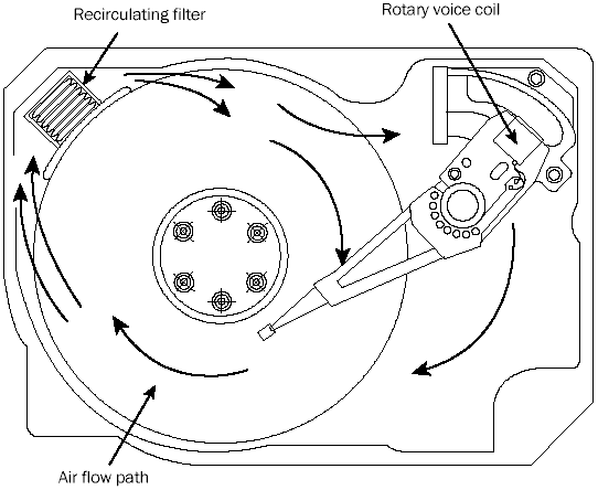
FIG. 1-6 Air circulation in a hard disk.
The HDA in a hard disk is sealed but not airtight. The HDA is vented through a barometric or breather filter element that allows for pressure equalization (breathing) between the inside and outside of the drive. For this reason, most hard drives are rated by the drive’s manufacturer to run in a specific range of altitudes, usually from -1,000 to +10,000 feet above sea level. In fact, some hard drives are not rated to exceed 7,000 feet while operating because the air pressure would be too low inside the drive to float the heads properly. As the environmental air pressure changes, air bleeds into or out of the drive so that internal and external pressures are identical. Although air does bleed through a vent, contamination usually is not a concern, because the barometric filter on this vent is designed to filter out all particles larger than 0.3 micron (about 12 µ-in) to meet the specifications for cleanliness inside the drive. You can see the vent holes on most drives, which are covered internally by this breather filter. Some drives use even finer-grade filter elements to keep out even smaller particles.
Hard Disk Temperature Acclimation
To allow for pressure equalization, hard drives have a filtered port to bleed air into or out of the HDA as necessary. This breathing also enables moisture to enter the drive, and after some period of time, it must be assumed that the humidity inside any hard disk is similar to that outside the drive. Humidity can become a serious problem if it is allowed to condense — and especially if the drive is powered up while this condensation is present. Most hard disk manufacturers have specified procedures for acclimating a hard drive to a new environment with different temperature and humidity ranges, especially for bringing a drive into a warmer environment in which condensation can form. This situation should be of special concern to users of laptop or portable systems with hard disks. If you leave a portable system in an automobile trunk during the winter, for example, it could be catastrophic to bring the machine inside and power it up without allowing it to acclimate to the temperature indoors.
The following text and Table 1.3 are taken from the factory packaging that Control Data Corporation (later Imprimis and eventually Seagate) used to ship its hard drives:
If you have just received or removed this unit from a climate with temperatures at or below 50°F (10°C) do not open this container until the following conditions are met, otherwise condensation could occur and damage to the device and/or media may result. Place this package in the operating environment for the time duration according to the temperature chart.
| Table 1.3 Hard Disk Drive Environmental Acclimation Table. | |
|---|---|
| Previous Climate Temp. | Acclimation Time |
| +40°F (+4°C) | 13 hours |
| +30°F (-1°C) | 15 hours |
| +20°F (-7°C) | 16 hours |
| +10°F (-12°C) | 17 hours |
| 0°F (-18°C) | 18 hours |
| -10°F (-23°C) | 20 hours |
| -20°F (-29°C) | 22 hours |
| -30°F (-34°C) or less | 27 hours |
As you can see from this table, a hard disk that has been stored in a colder-than-normal environment must be placed in the normal operating environment for a specified amount of time to allow for acclimation before it is powered on.
This is an archive of Alasir Enterprise’s MicroHouse PC Hardware Library Volume I: Hard Drives by Rhett M. Hollander (alasir.com) which disappeared from the internet in 2017. We wanted to preserve Rhett M. Hollander’s knowledge about hard drives and are permanently hosting a selection of important pages from alasir.com.